June 2026 · U.S. economy · Monthly recap
A price drop brought relief—with limits
Falling energy costs pulled the overall index down, while hiring was modest.
June delivered a change households could welcome: the overall consumer price index fell for the month. Energy costs played the biggest role. But the decline did not mean that all major expenses became cheaper, or that the cost of living had returned to its earlier level.
What happened to prices?
Consumer prices fell 0.4% over the month, after seasonal adjustment. The price basket was 3.5% higher than a year earlier, before seasonal adjustment. Energy fell 5.7%, while food rose 0.2%. BLS also reported increases in shelter. BLS price report.
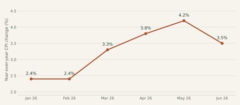
View the chart data and sources
| Month | Annual CPI | Source |
|---|---|---|
| January 2026 | 2.4% | BLS release ↗ |
| February 2026 | 2.4% | BLS release ↗ |
| March 2026 | 3.3% | BLS release ↗ |
| April 2026 | 3.8% | BLS release ↗ |
| May 2026 | 4.2% | BLS release ↗ |
| June 2026 | 3.5% | BLS release ↗ |
What happened to jobs?
The linked release reported 57,000 more nonfarm payroll jobs. The unemployment rate was 4.2%. BLS employment report.
What happened to interest rates?
The Federal Reserve held its target range at 3.50–3.75%. This is a benchmark for overnight bank lending, not the interest rate every consumer pays. Federal Reserve statement.
What this means in everyday life
A falling average can hide increases in individual categories. June’s report noted that food and shelter still rose while energy fell. Someone spending heavily on groceries or rent might therefore feel less relief than someone whose main pressure was fuel. The month is a good example of why the average basket and a personal budget are different.
One thing to keep in mind
The question was whether the energy decline would last. The jobs estimate also showed why it is useful to read prices and employment together: easier bills help, but income and opportunities remain part of financial security.
From the headlines to the classroom
AP Macro & Micro connections
Energy costs, supply shocks & production costs
AP Macro · Unit 3 · National Income and Price Determination
An increase in a widely used input cost can shift short-run aggregate supply left, raising the price level and reducing real output in the basic AD–AS model, all else equal. A cost decline can work in the opposite direction. The model helps explain a possible mechanism; CPI alone does not establish the cause of a real-world shock.
AP Micro · Unit 2 · Supply and Demand; 3 · Production, Cost, and the Perfect Competition Model
Fuel can be a variable input for a firm. A higher input price can raise marginal cost and reduce supply. However, the market price of fuel can also rise because demand increased, so a price change alone is not enough to identify a supply shift.
Try it yourself
Assume oil becomes more expensive because supply is disrupted. On an AD–AS graph with AD unchanged, what happens to SRAS, the price level, and real output?
Reveal the explanation
SRAS shifts left. The equilibrium price level rises and real output falls in the short run. Label the vertical axis Price level and the horizontal axis Real GDP, and show both equilibria. The supply disruption is an assumption in this question.
Sources & reporting notes
BLS Consumer Price Index — June 2026 ↗BLS Employment Situation — June 2026 ↗Federal Reserve decision — June 2026 ↗This is a retrospective, researched on October 6, 2026. Figures describe the month named above, unless a different period is stated. CPI and employment values are as reported in the linked archived releases; later revisions may differ. This recap focuses on prices, jobs, interest-rate decisions, and selected policy changes. It is educational, not personalized financial advice.
Check your understanding
The three-question quiz
One question about the recap, one about AP Macro, and one about AP Micro. These are original learning questions.